Sequencing Coverage
What is Coverage in NGS?
Next-generation sequencing (NGS) coverage describes the average number of reads that align to, or "cover," known reference bases. The sequencing coverage level often determines whether variant discovery can be made with a certain degree of confidence at particular base positions.
Sequencing coverage requirements vary by application, as noted below. At higher levels of coverage, each base is covered by a greater number of aligned sequence reads, so base calls can be made with a higher degree of confidence.
Sequencing Coverage Recommendations
Researchers typically determine the necessary NGS coverage level based on the method they're using, as well as other factors such as the reference genome size, gene expression levels, specific application of interest, published literature, and best practices from the scientific community. Examples of sequencing coverage recommendations for some common methods are listed here.
| Sequencing Method | Recommended Coverage |
|---|---|
| Whole genome sequencing (WGS) | 30× to 50× for human WGS (depending on application and statistical model) |
| Whole-exome sequencing | 100× |
| RNA sequencing | Usually calculated in terms of numbers of millions of reads to be sampled. Detecting rarely expressed genes often requires an increase in the depth of coverage. |
| ChIP-Seq | 100× |

How to Estimate and Achieve Your Desired NGS Coverage Level
Estimate Sequencing Runs:
The Lander/Waterman equation1 is a method for computing genome coverage. The general equation is: C = LN / G
- C stands for coverage
- G is the haploid genome length
- L is the read length
- N is the number of reads
We offer the following resources to help scientists determine coverage:
- Sequencing Coverage Calculator: Find out how to calculate the reagents and sequencing runs needed to achieve the desired sequencing coverage for your experiment
- RNA-Seq read length and coverage: Learn more about sequencing read depth guidelines for different RNA-Seq projects
When to Sequence More
You can increase coverage or sequence depth if you need more data. If necessary, combine the sequencing output from different flow cells along with your original sample. Here are some reasons to sequence more than your original estimated coverage:
- Adding statistical power to your assay
- Investigating very rare events
- Meeting minimum coverage thresholds for journals or fields
- Sequencing hard-to-sequence regions or polyploid genomes
Read Length Tips
Find out how to calculate the right read length for your sequencing run, and understand how NGS coverage is related to read length.
Learn MoreHistograms to Depict NGS Coverage Range and Uniformity
Coverage histograms are commonly used to depict the range and uniformity of sequencing coverage for an entire data set. They illustrate the overall coverage distribution by displaying the number of reference bases that are covered by mapped sequencing reads at various depths. Mapped read depth refers to the total number of bases sequenced and aligned at a given reference base position (note that "mapped" and "aligned" are used interchangeably in the sequencing community).
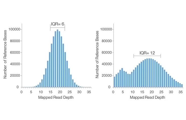
In a sequencing coverage histogram, the read depths are binned and displayed on the x-axis, while the total numbers of reference bases that occupy each read depth bin are displayed on the y-axis. These can also be written as percentages of reference bases.
Examples of Coverage Histograms
Ideally, the plot will take the form of a Poisson-like distribution with a small standard deviation, as seen in this histogram image. This distribution is valid under the assumption that reads are randomly distributed across the genome and that the ability to detect true overlaps between reads is constant within a sequencing run.
However, for a variety of reasons, actual coverage histograms may have a large spread (i.e., broad range of read depths), or have a non-Poisson distribution, as seen in the right-hand example of a poor sequencing coverage histogram.
Evaluating Next-Generation Sequencing Coverage
The following metrics are commonly used to evaluate NGS coverage:
Inter-Quartile Range (IQR)
The IQR is the difference in sequencing coverage between the 75th and 25th percentiles of the histogram. This value is a measure of statistical variability, reflecting the non-uniformity of coverage across the entire data set.
A high IQR indicates high variation in coverage across the genome, while a low IQR reflects more uniform sequence coverage. In the example histograms above, the lower IQR indicates that the histogram on the left has better sequencing coverage uniformity than that on the right.
Mean (Mapped) Read Depth
The mean mapped read depth (or mean read depth) is the sum of the mapped read depths at each reference base position, divided by the number of known bases in the reference.
The mean read depth metric indicates how many reads, on average, are likely to be aligned at a given reference base position.
Raw Read Depth
This is the total amount of sequence data produced by the instrument (pre-alignment), divided by the reference genome size. Although raw read depth is often provided by sequencing instrument vendors as a specification, it does not take into account the efficiency of the alignment process.
If a large fraction of the raw sequencing reads are discarded during the alignment process, the post-alignment mapped read depth can be significantly smaller than the raw read depth.
Interested in receiving newsletters, case studies, and information from Illumina based on your area of interest? Sign up now.
Reference
- Lander ES, Waterman MS. Genomic mapping by fingerprinting random clones: a mathematical analysis. Genomics. 1988;2(3):231-239. doi:10.1016/0888-7543(88)90007-9